1. Overview
Every company has a challenge of matching its supply volume to a customer demand. How well a company manages this challenge has a major impact on its profitability. The typical cost of carrying inventory is at least 10.0 percent of the inventory value. So, the amount of inventory held has a major impact on available cash. It is important for companies to keep inventory levels as low possible and to sell inventory as quickly as possible. Studies have shown a significant correlation between overall manufacturing profitability and inventory turns. The challenge of managing inventory is increased by the “long tail” phenomenon which is causing a greater percentage of total sales for many companies to come from a large number of products, each with low sales frequency. Shorter and more frequent product cycles which are required to meet the needs of more sophisticated markets create the need to manage supply chains containing more products and parts.
In many cases we deal with multi-echelon structure of supply chain with a few upstream and downstream facilities combined in a complex network structure (see Section II.2 below). Modeling and optimization of multi-echelon supply chain systems is challenging as it requires a holistic approach that exploits interactions between echelons while accurately accounting for variability observed by these systems. However, it provides most effective solution for lowering overall inventory cost, and increasing safety stock levels across all of these echelons.
Price optimization for goods sold by retailer stores is another important aspect of supply chain optimization. It is discussed in detail in Section II.3.
Due its complex structure, a supply chain network requires sophisticated and quick algorithms to optimize logistics. This topic is covered in Section II.4.
Modern technologies based on integration of Artificial Intelligence (AI), Machine Learning (ML), and optimization algorithms allow us to solve most of such problems in an effective way. They include learning from time series of historical data with all possible factors included. Using this data one can train models that would be able to predict optimal stocking, and minimize operation costs.
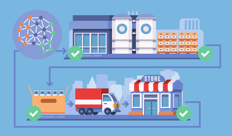
Figure 1: Supply Chain.
To summarize, typical data science applications in the supply chain problem include
- predicting demand on different items
- multi-echelon inventory optimization
- price optimization
- managing logistical relationship between the supply chain nodes
2. Forecasting demand
In this problem, we need to predict optimal number of stock-keeping units (SKUs) we should keep at a given facility to satisfy customer needs. Let’s say, we would like to know how many bottles of milk X we need to keep in a particular store Y next week. Typical approaches include introduction of some safety buffer (let’s say, 20-30% are added) to a projected quantity. However, the amount of SKU you manage to sell turns out to be close to the initial forecast and the company ends up with overstock. Another approach may be based on some “known” probability distribution for a demand. But this assumption is often far been optimal because it may not take into account a number of important factors which leads to a significant bias in predictions. Most advanced technique is based on application of Machine learning techniques based on deep learning with neural networks, DNN (see Fig.2).
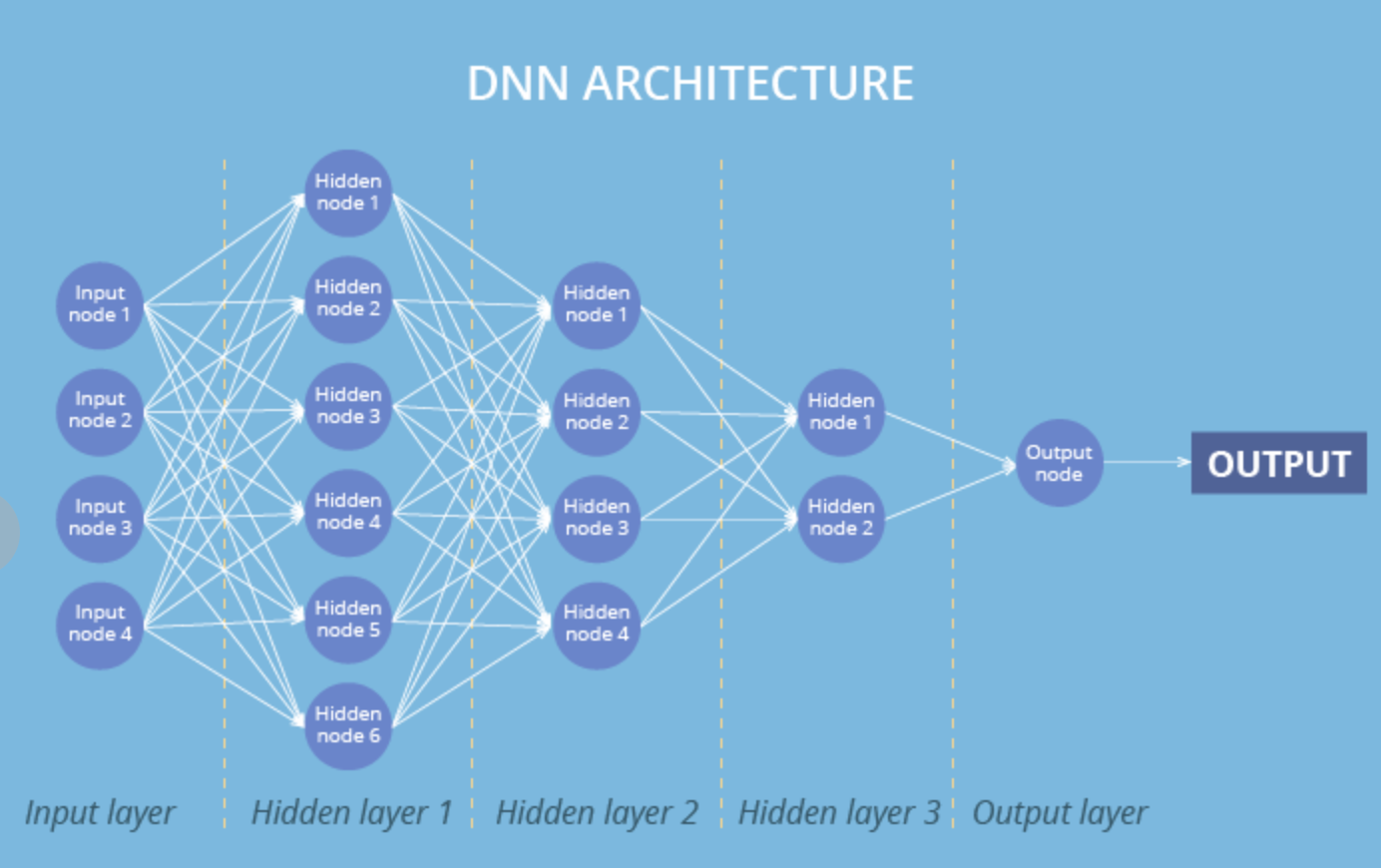
Figure 2: Typical Deep Neural Net architecture.
In this case we do not need to guess about a “core” probability distribution. Instead, we forecast using historical sales and all the factors that should affect the demand. It may include last N days of sales, week of year (seasonality), day of week, item category, store type, promotion, holidays, etc. The neural network trained on historical data, is able to learn patterns and trends that might be hidden and not clear at a first sight. After such training, DNN predicts demand/sales as a function of a number of all the factors (Fig.3). As a result, predicted demand becomes dynamic (as it should be). It also means that amount of goods we keep becomes more precise, i.e. much more efficient in a financial sense. In its turn, it may require a more dynamic supply chain as well.
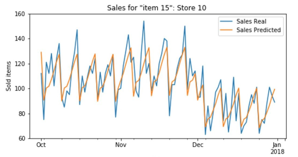
Figure 3: Prediction of sales using time series data and DNN.
3. Multi-echelon inventory optimization
In many cases, a supply chain has a complex structure with multiple facilities with a sequential supply structure, i.e. has a few echelons. Figure 4 illustrates an example of such multi-echelon supply chain network. The network comprises both elements of a multi-echelon system where a stocking facility can either purely serve customer demand or just replenishes another facility, or does a combination of both. In Fig. 4, the outermost stocking facilities 2, 4, and 5 are customer facing units that directly serve customer demand. Stocking facility 1 is a central facility that, besides directly fulfilling customer orders, also replenishes facility 2. Facility 3 is another c entral facility that mainly replenishes 4 and 5. It gets its replenishment from the first facility. The first node that replenishes facility 1 is a supply node, such as a manufacturing plant or a vendor, for which we do not track inventory. Thus, facility 3 has no explicit target; though it can centrally keep inventory for nodes 4 and 5 in order to facilitate meeting their service level targets. The time gap between placing orders and receiving replenishment is characterized by an overall lead time.
In this case, the purpose of inventory optimization is to minimize total system costs. This can include order placement cost, inventory holding cost, and other miscellaneous charges such as facility costs, etc. A good optimization algorithm, being cognizant of the entire system, optimizes all echelons simultaneously.
Such optimization is a difficult problem, for which accurate capturing interactions and dynamics is paramount. A few mathematical methods exist. They are based on modeling processes (simulation) at different stages, such as placing, fulfilling, shipping order, and serving customer demand using historical data. The objective function has two components that the solver seeks to minimize. The first component is the total of average on-hand inventory of all facilities, while the second is the penalty for not meeting the service level targets summed across all facilities.
The goal of multi-echelon inventory optimization is to continually update and optimize safety stock levels across all of these echelons. Multi-echelon inventory optimization represents the state of the art approach to optimize inventory across the end to end supply chain.
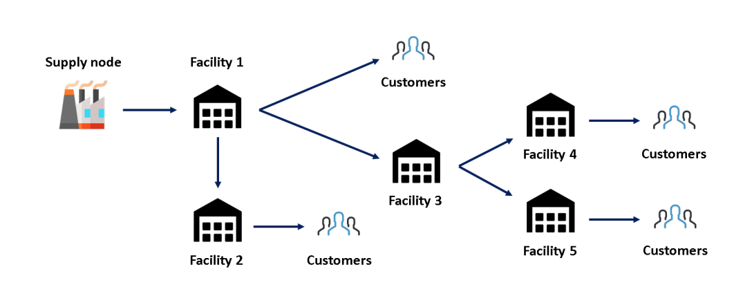
Figure 4: A multi-echelon supply chain example.
4. Price optimization
Here are some of the crucial questions that retailers recurrently face:
- What price should we set if we want to make the sale in less than a week?
- What is the fair price of this product, given the current state of the market, the period of the year, the competition, or the fact that it is a rare product?
Retailers must pay close attention to several parameters when setting prices. Factors such as competition, market positioning, production costs, and distribution costs, play a key role for retailers in order to make the right move. ML can be of great help in this case and have an enormous impact on KPIs. Its power lies in the fact that the developed algorithms can learn patterns from data, instead of being explicitly programmed. ML models can continuously integrate new information and detect emerging trends or new demands into predictive models. Retailers can benefit from the predictive models that allow them to determine the best price for each product or service.
Price optimization techniques can help retailers evaluate the potential impact of sales promotions or estimate the right price for each product if they want to sell it in a certain period of time. Current state-of-the-art techniques in price optimization allow retailers to consider factors such as:
- Competition
- Weather
- Season
- Operating costs
- Local demand
- Company objectives
To train ML models, it is necessary to have different kinds of information, such as:
- Transactional: a sales history that includes the list of the products purchased and, eventually, the customers who purchased them.
- Description of the products: a catalog with relevant information about each product such as category, size, brand, style, color, photos and manufacturing or purchase cost.
- Data on past promotions and past marketing campaigns.
- Customer Reviews: reviews and feedback given by customers about the products.
- Data on the competition: prices applied to identical or similar products.
- Inventory and supply data.
- In the case of physical stores: information about their geographical location and that of the competitors.
It is important to define the strategic goals and constraints. Retailers may pursue a unique, clear objective of profit maximization. However, they may also be interested in customer loyalty (e.g. increasing the net promoter score or the conversion rate) or in attracting a new segment (e.g. young people). Price optimization with ML has clear advantages. First of all, it is automation and speed of all predictions. Second, ML models can consider a huge number of products and optimize prices globally. For example, it is known that changing the price of a product often impacts the sales of other products in ways that are very hard to predict for a human. In most cases, the accuracy of a ML solution will be significantly higher than that of a human. In addition, retailers can modify the KPI and immediately see how the models recalculate prices for the new goals. Third, by analyzing a large amount of past and current data, a ML can anticipate trends early enough. This is a key issue that allows retailers to make appropriate decisions to adjust prices. Finally, in the case of a competitive pricing strategy, ML solutions can continuously crawl the web and social media to gather valuable information about prices of competitors for the same or similar products, what customers say about products and competitors, considering hot deals, as well as the price history over the last number of days or weeks.
Price optimization helps retailers understand how customers will react to different price strategies for products and services, and set the best prices. ML models can take key pricing variables into account (e.g. purchase histories, season, inventory, competitors’ pricing), to find the best prices, even for vast catalogs of products or services, that can achieve the set KPIs. These models don’t have to be programmed. They learn patterns from data and are capable of adapting themselves to new data. They allow retailers to quickly test different hypotheses and make the best decision.
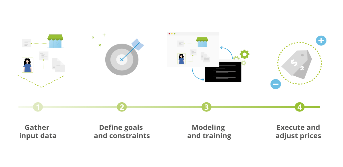
Figure 5: Process of defining prices in retail with price optimization using Machine Learning.
5. Managing logistical relationship between the supply chain nodes
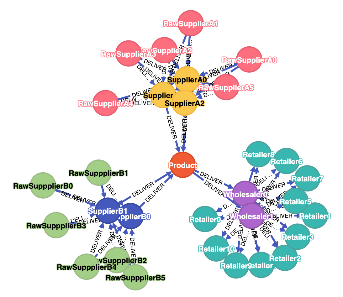
Supply chains are inherently complex and can be modeled and clustered in several different ways. In order to model and understand supply chains better, many sources refer to modern supply chains as networks. Therefore, it is a perfect environment to apply modern graphical data bases to help us resolve many supply chain network challenges.
Example supply chain is shown on Fig.5. We can categorize our suppliers into RawSupplier A and Supplier A for fresh products and RawSupplier B and Supplier B for durable commodities. The rest is straight forward. The distribution is through wholesaler and retailer. Distance between connected nodes can be based on the longitude and latitude.
Using graphical representation and modern graph/network algorithms, many problems can be solved quite easily. For example, for the network in Fig.5, for each Wholesaler one can find the least accumulated distance to every retailer. If we know quality of all items distributed by RawSuppliers (e.g. freshness), we can find optimal supply chains (routes) to have them delivered to Retailers within a given amount of time. We can also find just local product suppliers who are just within X miles from a retailer. One can also introduce some score for each supply chain route, e.g. in terms of cost, time and amount of waste. Total score can be used as a KPI which eases complex decision-making and quick comparison. The total score also comes in handy in case we want to diminish the number of our (raw) supplier and only retain the top performer.
Due to the nature of supply chains, which is inherently a graph or network structure, graph databases and algorithms are more suitable to monitor, maintain and model supply chain problems e.g. Risk Management, Transport Optimization, and quality assurance.